There are two summary functions included with the rCISSVAE package that can help visualize the data clusters and model suitability to the data.
Per-cluster Summary
The cluster_summary() function creates a data summary
table stratified by missingness cluster. The function builds on
gtsummary::tbl_summary(), so gtsummary-like statistics can
be used for summarizing variables
(
see tbl_summary() documentation for details ).
## ── Attaching core tidyverse packages ──────────────────────── tidyverse 2.0.0 ──
## ✔ dplyr     1.1.4     ✔ readr     2.1.5
## ✔ forcats   1.0.0     ✔ stringr   1.6.0
## ✔ ggplot2   4.0.1     ✔ tibble    3.3.0
## ✔ lubridate 1.9.4     ✔ tidyr     1.3.2
## ✔ purrr     1.2.0
## ── Conflicts ────────────────────────────────────────── tidyverse_conflicts() ──
## ✖ dplyr::filter() masks stats::filter()
## ✖ dplyr::lag()    masks stats::lag()
## ℹ Use the conflicted package (<http://conflicted.r-lib.org/>) to force all conflicts to become errors##
## Attaching package: 'kableExtra'
##
## The following object is masked from 'package:dplyr':
##
## group_rows
library(gtsummary)

data(df_missing)
data(clusters)

## Integer clusters must be passed in as a factor
cluster_summary(data = df_missing, factor(clusters$clusters),
include = setdiff(names(df_missing), "index"),
statistic = list(
  all_continuous() ~ "{mean} ({sd})",
  all_categorical() ~ "{n} / {N}\n ({p}%)"),
missing = "always")| Characteristic | N |
0 N = 2,0001 |
1 N = 2,0001 |
2 N = 2,0001 |
3 N = 2,0001 |
|---|---|---|---|---|---|
| Age | 8,000 | 10.10 (2.04) | 10.19 (2.08) | 10.21 (2.14) | 10.29 (2.06) |
| Unknown | 0 | 0 | 0 | 0 | |
| Salary | 8,000 | 5.81 (0.61) | 5.83 (0.62) | 5.83 (0.61) | 5.81 (0.60) |
| Unknown | 0 | 0 | 0 | 0 | |
| ZipCode10001 | 8,000 | 646 / 2,000 (32%) | 674 / 2,000 (34%) | 663 / 2,000 (33%) | 645 / 2,000 (32%) |
| Unknown | 0 | 0 | 0 | 0 | |
| ZipCode20002 | 8,000 | 703 / 2,000 (35%) | 652 / 2,000 (33%) | 655 / 2,000 (33%) | 687 / 2,000 (34%) |
| Unknown | 0 | 0 | 0 | 0 | |
| ZipCode30003 | 8,000 | 651 / 2,000 (33%) | 674 / 2,000 (34%) | 682 / 2,000 (34%) | 668 / 2,000 (33%) |
| Unknown | 0 | 0 | 0 | 0 | |
| Y11 | 4,878 | -21 (10) | -16 (9) | 8 (5) | -3 (6) |
| Unknown | 1,281 | 1,288 | 0 | 553 | |
| Y12 | 4,882 | 69 (11) | -26 (9) | 55 (6) | -24 (8) |
| Unknown | 1,264 | 1,283 | 0 | 571 | |
| Y13 | 4,890 | 77 (12) | -25 (9) | 98 (12) | -17 (7) |
| Unknown | 1,289 | 1,264 | 0 | 557 | |
| Y14 | 4,871 | 73 (12) | -21 (8) | 125 (16) | -11 (6) |
| Unknown | 1,300 | 1,283 | 0 | 546 | |
| Y15 | 4,859 | 76 (12) | -12 (6) | 141 (19) | -14 (6) |
| Unknown | 1,273 | 1,293 | 0 | 575 | |
| Y21 | 4,865 | -33 (12) | -28 (11) | 1 (7) | -12 (7) |
| Unknown | 1,266 | 1,292 | 0 | 577 | |
| Y22 | 4,906 | 69 (12) | -40 (12) | 54 (6) | -36 (10) |
| Unknown | 1,266 | 1,276 | 0 | 552 | |
| Y23 | 4,902 | 79 (13) | -38 (11) | 104 (13) | -29 (9) |
| Unknown | 1,273 | 1,275 | 0 | 550 | |
| Y24 | 4,854 | 75 (12) | -32 (10) | 135 (18) | -22 (7) |
| Unknown | 1,302 | 1,287 | 0 | 557 | |
| Y25 | 4,894 | 78 (13) | -22 (8) | 153 (21) | -25 (8) |
| Unknown | 1,257 | 1,294 | 0 | 555 | |
| Y31 | 5,933 | -18 (10) | -13 (9) | 13 (5) | 1 (6) |
| Unknown | 192 | 1,285 | 0 | 590 | |
| Y32 | 5,944 | 74 (11) | -24 (10) | 62 (7) | -21 (8) |
| Unknown | 206 | 1,287 | 0 | 563 | |
| Y33 | 5,987 | 84 (13) | -23 (10) | 108 (13) | -14 (7) |
| Unknown | 203 | 1,267 | 0 | 543 | |
| Y34 | 5,949 | 81 (13) | -17 (8) | 136 (17) | -7 (6) |
| Unknown | 195 | 1,275 | 0 | 581 | |
| Y35 | 5,946 | 83 (13) | -8 (6) | 153 (20) | -10 (7) |
| Unknown | 204 | 1,285 | 0 | 565 | |
| Y41 | 5,968 | -8 (4) | -5 (3) | 6 (2) | 1 (2) |
| Unknown | 184 | 1,279 | 0 | 569 | |
| Y42 | 5,978 | 35 (6) | -11 (4) | 29 (4) | -9 (3) |
| Unknown | 199 | 1,282 | 0 | 541 | |
| Y43 | 5,987 | 39 (7) | -10 (3) | 49 (6) | -6 (3) |
| Unknown | 217 | 1,242 | 0 | 554 | |
| Y44 | 5,977 | 37 (7) | -8 (3) | 62 (9) | -3 (2) |
| Unknown | 186 | 1,280 | 0 | 557 | |
| Y45 | 5,914 | 39 (7) | -4 (3) | 70 (10) | -5 (2) |
| Unknown | 204 | 1,305 | 0 | 577 | |
| Y51 | 5,923 | -5.4 (3.6) | -2.9 (3.0) | 6.9 (1.9) | 2.5 (2.0) |
| Unknown | 222 | 1,279 | 0 | 576 | |
| Y52 | 5,966 | 32 (5) | -8 (3) | 26 (3) | -6 (3) |
| Unknown | 209 | 1,283 | 0 | 542 | |
| Y53 | 6,024 | 35 (6) | -6 (3) | 44 (6) | -3 (2) |
| Unknown | 184 | 1,243 | 0 | 549 | |
| Y54 | 5,953 | 34 (6) | -5 (3) | 55 (7) | -1 (2) |
| Unknown | 217 | 1,281 | 0 | 549 | |
| Y55 | 5,950 | 35 (6) | -2 (2) | 62 (9) | -2 (2) |
| Unknown | 207 | 1,292 | 0 | 551 | |
| 1 Mean (SD); n / N (%) | |||||
Missingness Heatmap
cluster_heatmap(
  data = df_missing,
  clusters = paste0("Cluster ", clusters$clusters), ## Adds 'Cluster' to the cluster label
  cols_ignore = "index",
  observed_color = "#23013aff", ## A dark purple
  missing_color = "yellow")
## `use_raster` is automatically set to TRUE for a matrix with more than
## 2000 columns You can control `use_raster` argument by explicitly
## setting TRUE/FALSE to it.
##
## Set `ht_opt$message = FALSE` to turn off this message.## 'magick' package is suggested to install to give better rasterization.
##
## Set `ht_opt$message = FALSE` to turn off this message.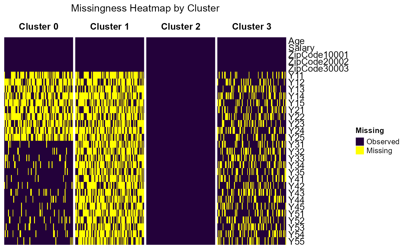
By-cluster imputation loss function
After running the model, you can get the per-cluster validation set
imputation loss using the performance_by_cluster()
function. Set ‘return_validation_dataset = TRUE’ in the
run_cissvae() function to be able to use
performance_by_cluster on the result object. If the validation dataset
(val_data in result object) and imputed validation dataset (val_imputed
in the result object) are not returned, the imputation loss cannot be
calculated.
If the run_cissvae() function was used to generate
clusters, set return_clusters=TRUE and the clusters will be
part of the return object. Otherwise, use the ‘clusters’ parameter in
performance_by_cluster() to input the clusters.
result = run_cissvae(
  data = df_missing,
  index_col = "index",
  val_proportion = 0.1, ## pass a vector for different proportions by cluster
  columns_ignore = c("Age", "Salary", "ZipCode10001", "ZipCode20002", "ZipCode30003"), ## If there are columns in addition to the index you want to ignore when selecting validation set, list them here. In this case, we ignore the 'demographic' columns because we do not want to remove data from them for validation purposes.
  clusters = clusters$clusters, ## we have precomputed cluster labels so we pass them here
  epochs = 5,
  return_silhouettes = FALSE,
  return_history = TRUE,  # Get detailed training history
  verbose = FALSE,
  return_model = TRUE, ## Allows for plotting model schematic
  device = "cpu",  # Explicit device selection
  layer_order_enc = c("unshared", "shared", "unshared"),
  layer_order_dec = c("shared", "unshared", "shared"),
  return_validation_dataset = TRUE
)

cat(paste("Check necessary returns:", paste0(names(result), collapse = ", ")))
## Check necessary returns: imputed_dataset, model, clusters, training_history, val_data, val_imputed
feature_cols = setdiff(
  names(result$val_data),
  c("index", "Age", "Salary", "ZipCode10001", "ZipCode20002", "ZipCode30003")
)
performance_by_cluster(res = result,
  group_col = NULL,
  clusters = clusters$clusters,
  feature_cols = feature_cols,
  by_group = FALSE,
  by_cluster = TRUE,
  cols_ignore =  c( "index", "Age", "Salary", "ZipCode10001", "ZipCode20002", "ZipCode30003"), ## columns to not score
  )
## $overall
## mse bce ce accuracy imputation_error
## 1 60.73548 NA NA NA 60.73548
##
## $per_cluster
## cluster mse bce ce accuracy imputation_error
## 1 0 39.97412 NA NA NA 39.97412
## 2 1 98.66703 NA NA NA 98.66703
## 3 2 56.52029 NA NA NA 56.52029
## 4 3 67.43755 NA NA NA 67.43755